Visual Features of Sheet Music Using Autoencoders
Format (When): Where
- Presentation (2025): International Conference on Computational and Cognitive Musicology
Dataset
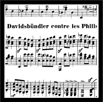
I collected sheet music from 7 musical periods, 3 composers from each period. Pieces are separated by composer, and are split into individual pages as jpgs. A minimum of 30 pages of music was ensured for each composer. The dataset includes 1,302 pages of music from 101 pieces. To train the model, I isolated 5 random (448x448 px) samples from each image (meaning there are 6,510 samples)—see below. To ensure samples were not predominantly white, I used a whiteness threshold (.9) to exclude samples which have a mean pixel value considered too white.
Because I included popular music and scans that are not in the public domain, I am choosing not to publicly share the dataset—I am happy to give access to anyone who would like to see it or use it for research purposes.
| Styles | 7 : (Baro., Class., Rom., Impress., Rag., Tin-Pan, Pop/Rock) |
|---|---|
| Composers/Artists | 21 (3 from each style) |
| Pages | 1302 (min 30 from each) |
| Pieces | 101 |
| Samples | 6,510: 5 (448 x 448) samples from each score. |


Model Architecture
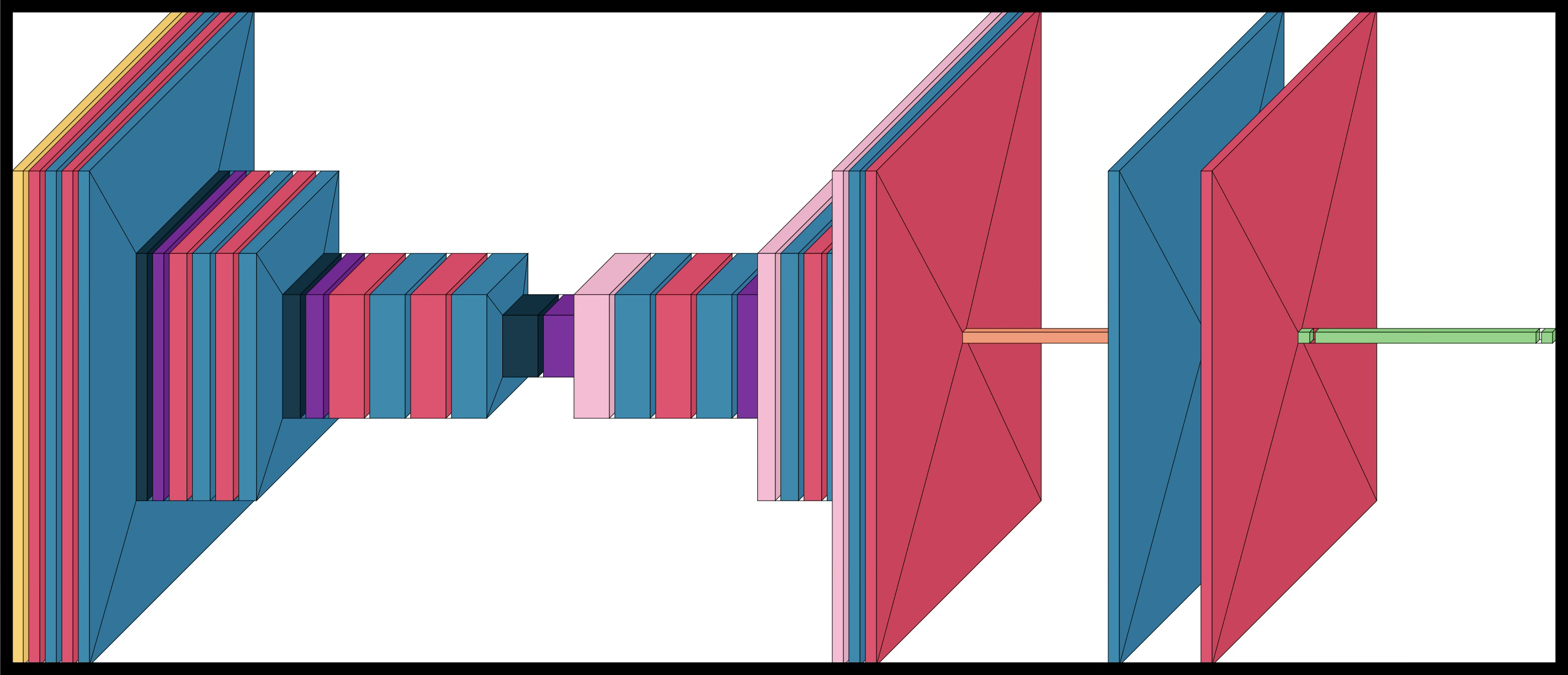
 The model is a convolutional autoencoder with a classification head. Unpacking that a bit:
An autoencoder is an unsupervised neural network model composed of an 1) encoder, 2) bottleneck (or latent space), and 3) decoder. The goal of the model is to produce an output that matches the input _\hat{x}≈_x where x is the input and \hat{x} is the reconstruction. However, we reduce the input to a lower dimmension—we reduce the image from 448x448 px to, ultimately, 56x56 px. (It gets reduced to 224x224 and 112x112 along the way.) The job of the encoder is to reduce the image to a 56x56 px image—which is known as the bottleneck—and the job of the decoder is to reproduce the original image by upsampling from its smaller state.
For the convolution, we take a 5x5 or 3x3 filter and slide it across the image—one example of a filter is shown below. We take the dot product between the filter and the image (multiplying each position with the position beneath it and summing those values). By continuing to slide the filter across the image, it results in a new matrix showing where the filter “matched” the image. After training, filters learn and correspond to certain features of the image to better compress or reproduce the image. Typically, filters in the earlier stages of the autoencoder correspond to basic visual features, and those later learn more sophisticated representations.

In the model above, I have also added batch normalization and dropout. Batch normalization shifts the mean of the output layer to be close to 0 and the standard deviation close to 1. Dropout randomly “drops” (sets to zero) a fraction of layer outputs during training to prevent the model from overfitting to the training dataset. The rate used was a standard 0.25, meaning 25% of connections are dropped.
The actual filter looks like this: |(5x5)x16|(3x3)x32|(3x3)x64| There are 3 layers 16 of 5x5 filters, 3 layers of 32 3x3 filters, and 3 layers of 64 3x3 filters.
The classification head is added to the bottleneck of the model and I don’t use it for this project. Message me for details.
Training
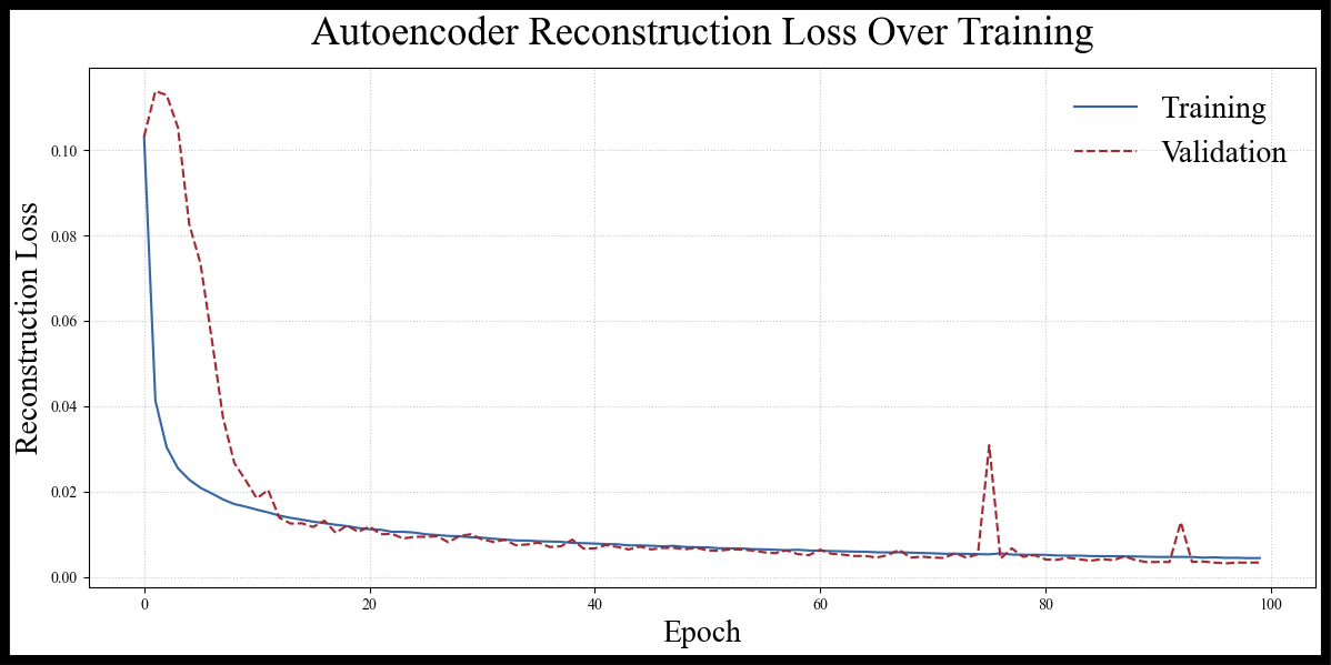
The model is evaluated based on how similar the reconstructed image is to the original---the error is known as Mean Squared Error (MSE). MSE is just the averaged squared distance between the original and reconstructed image.
Then, like most neural networks, we use backpropagation for updating our model. Based on the error, gradients flow back through all paths, and the Adam optimizer updates the filters to minimize the MSE.
The actual parameters are below:
- 100 epochs (loops through the dataset)
- Batch size of 32
- Dropout (0.25) used throughout for regularization
- Batch normalization after convolutions
- Validation on 20% held-out test set
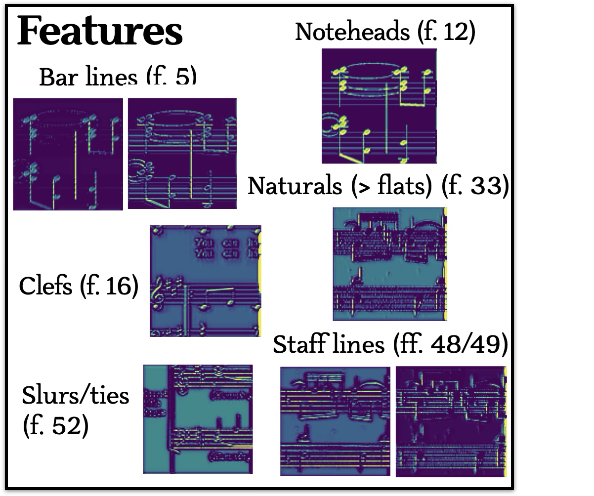
Visual features
After training the model, it achieved minimal error in its reconstruction of the image (and was not overfit to the training dataset). By examining the latent space, we can see what the model thinks is the most essential to an images construction. Below find some recurring filters.
References
Balke, S., Achankunju, S. P., & Müller, M. (2015). Matching musical themes based on noisy OCR and OMR input. In Proceedings of the IEEE International Conference on Acoustics, Speech, and Signal Processing (ICASSP), 703–707. https://doi.org/10.1109/ICASSP.2015.7178060
Byrd, D., & Simonsen, J. G. (2015). Towards a standard testbed for optical music recognition: Definitions, metrics, and page images. Journal of New Music Research, 44(3), 169–195. https://doi.org/10.1080/09298215.2015.1045424
Chiu, M., & Temperley, D. (2024). Melodic Differences Between Styles: Modeling Music with Step Inertia. Music and Science 7. https://doi.org/10.1177/20592043231225731
Conklin, D., & Witten, I. H. (1995). Multiple viewpoint systems for music prediction. Journal of New Music Research, 24(1), 51–73. https://doi.org/10.1080/09298219508570672
Hajic Jr, J., Pecina, P., et al. (2017). The MUSCIMA++ dataset for handwritten optical music recognition. In International Conference on Document Analysis and Recognition (ICDAR) (pp. 39–46). https://doi.org/10.1109/ICDAR.2017.16
Herremans, D., Chuan, C. H., & Chew, E. (2017). A functional taxonomy of music generation systems. ACM Computing Surveys (CSUR), 50(5), 1–30. https://doi.org/10.1145/3108242
Masci, J., Meier, U., Cireşan, D., & Schmidhuber, J. (2011). Stacked convolutional auto-encoders for hierarchical feature extraction. In International Conference on Artificial Neural Networks (pp. 52–59). Springer. https://doi.org/10.1007/978-3-642-21735-7_7
McKay, C., & Fujinaga, I. (2006). Musical genre classification: Is it worth pursuing and how can it be improved? In Proceedings of the International Society for Music Information Retrieval Conference (ISMIR 2006).
Pons, J., Lidy, T., & Serra, X. (2017). Experimenting with musically motivated convolutional neural networks. In 14th International Workshop on Content-Based Multimedia Indexing (pp. 1–6). https://doi.org/10.1109/CBMI.2016.7500246
Rebelo, A., Fujinaga, I., Paszkiewicz, F., Marcal, A. R. S., Guedes, C., & Cardoso, J. S. (2012). Optical music recognition: State-of-the-art and open issues. International Journal of Multimedia Information Retrieval, 1(3), 173–190. https://doi.org/10.1007/s13735-012-0004-6
Sigtia, S., Kumar, S., Mauch, M., Benetos, E., & Dixon, S. (2016). An end-to-end neural network for polyphonic piano music transcription. IEEE/ACM Transactions on Audio, Speech, and Language Processing, 24(5), 927–939. https://doi.org/10.1109/TASLP.2016.2535164